Single-Shot Mueller Matrix Polarimetry Using a Multichannel Lock-In with Four Reference Frequencies

This application note describes how SynkTek MCL1-540 multichannel lock-in amplifier measurment system with four reference frequency outputs can be used to measure the full 4×4 Mueller matrix of an optical sample in a single static acquisition. By driving four photoelastic modulators (PEMs) at distinct frequencies and demodulating the detected intensity at eight derived frequencies, the 16 real Mueller matrix elements are recovered via linear inversion. The approach enables drift-free, high-SNR polarimetry with no moving parts.

1. Introduction

Mueller matrix polarimetry characterizes the complete polarization response of an optical sample, including diattenuation, retardance, and depolarization. Traditional implementations rely on rotating optical elements or sequential polarization states, which are sensitive to drift and limit temporal resolution.

A 4-PEM polarimeter, combined with a multichannel lock-in amplifier, enables simultaneous encoding of all Mueller matrix elements into distinct Fourier components of the detected intensity. The lock-in’s ability to reference multiple frequencies simultaneously and demodulate multiple harmonics is central to this method.

2. System Overview

2.1 Optical configuration

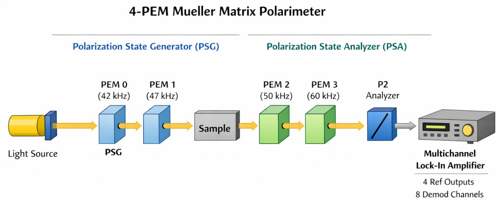
A typical 4-PEM Mueller polarimeter consists of:

• Polarization State Generator (PSG)
  • Linear polarizer P₁
  • PEM₀ driven at frequency $f_0$
  • PEM₁ driven at frequency $f_1$
• Sample under test
• Polarization State Analyzer (PSA)
  • PEM₂ driven at frequency $f_2$
  • PEM₃ driven at frequency $f_3$
  • Linear polarizer P₂
  • Photodetector

Each PEM is operated at a fixed retardance amplitude and a fixed fast-axis azimuth.

2.2 Lock-in configuration

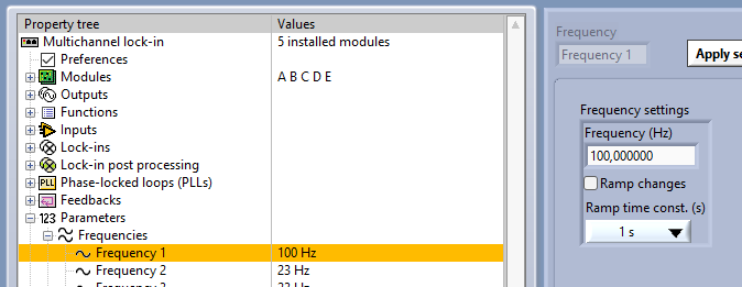
The MCL1-540 lock-in amplifier system provides:

• Four phase-coherent reference outputs on modules A, B, C and D:
  Used to drive the PEM controllers at four frequencies, for example: $$f_0 = 42\text{ kHz},\quad f_1 = 47\text{ kHz},\quad f_2 = 50\text{ kHz},\quad f_3 = 60\text{ kHz}$$
• One detector signal analog input, module A V1
• Eight demodulation channels, each capable of:
  • Arbitrary reference frequency selection
  • In-phase (X) and quadrature (Y) detection
  • Phase-coherent averaging

The detector signal is connected to a single analog input; all polarization information is demodulated in the instrument.

Drive PEM₀ by the output of module A, PEM₁ by the output of module B, PEM₂ by the output of module C, and PEM₃ by the output of module D.

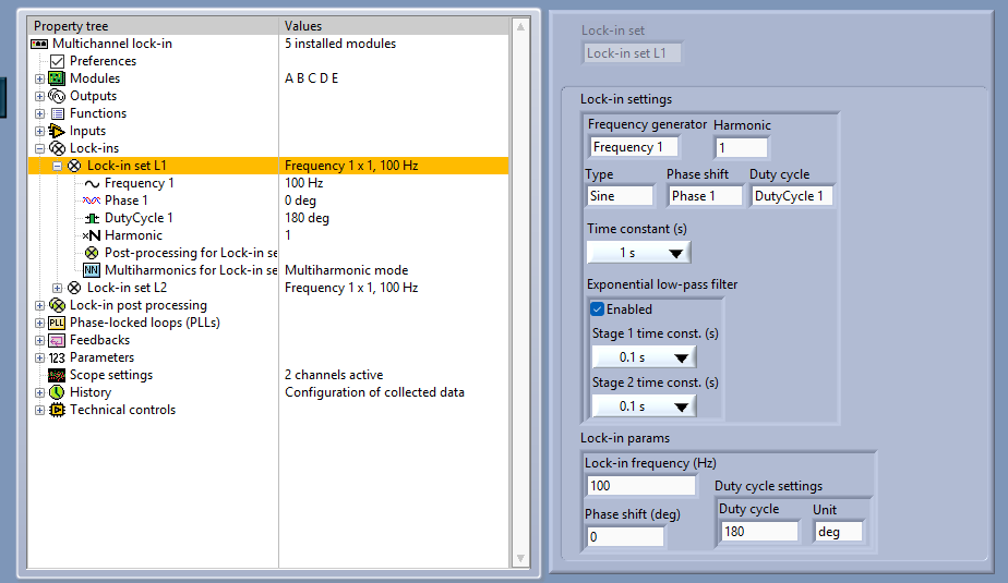
Configure Frequency 1 to 100 Hz, all other frequencies will be derived as harmonics from this frequency to achieve phase coherence:

Configure the output of module A as Function 1, based on Frequency 1 at harmonic 420. Since Frequency 1 is at 100Hz, the output will be driven at a frequency of (420 x 0.100 = 42) kHz. Choose a suitable amplitude for driving PEM₀, in this example 1 V>

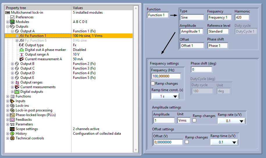
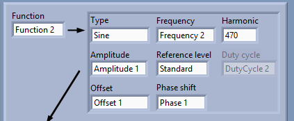
Set up the other outputs B-D in a similar way, i.e. output B as Function 2, but based on Frequency 1 with Harmonic 470:

Configure input A V1 with appropriate gain settings, use DC coupling.

Configure Lock-in set L1 to be based on Frequency 1 on harmonics 1:

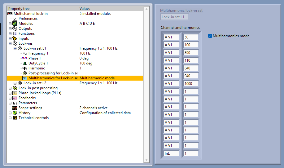
Enable the multiharmonics mode and set the harmonics of the demodulators so that the harmonics of 100Hz matches frequencies according to the table in section 4. Note that only 7 channels are used and frequencies are configured since the DC value, channel 1 in the table, is always calculated independent of the selected harmonics:

3. Measurement Principle

3.1 Intensity as a linear function of the Mueller matrix

The detected intensity can be written as:$$I(t) = \mathbf{A}^T(t)\, \mathbf{M}\, \mathbf{G}(t)$$where:

• $\mathbf{M}$ is the 4×4 Mueller matrix of the sample,
• $\mathbf{G}(t)$ is the time-dependent Stokes vector generated by the PSG,
• $\mathbf{A}^T(t)$ is the time-dependent analyzer row vector of the PSA.

Expanding this expression yields:$$I(t) = \sum_{p=0}^{3}\sum_{q=0}^{3} m_{pq}\, z_{pq}(t)$$with known basis functions:$$z_{pq}(t) = A_p(t)\,G_q(t)$$Thus, the measured signal is a linear superposition of 16 known time-dependent basis functions, weighted by the Mueller matrix elements.

3.2 Frequency encoding via PEM modulation

Each PEM introduces a retardance:$$\delta_i(t) = \delta_{0i}\sin(2\pi f_i t + \phi_i)$$The resulting trigonometric terms expand into Fourier series containing harmonics of $f_i$​. Products of PSG and PSA terms generate sum and difference frequencies of the form:$$f = \pm n_0 f_0 \pm n_1 f_1 \pm n_2 f_2 \pm n_3 f_3$$By choosing four distinct PEM frequencies, many of these combinations are spectrally isolated and can be measured independently.

4. Demodulation Strategy

4.1 Why eight demodulation frequencies are sufficient

Each demodulation channel yields two real values:

• In-phase component $X_k$
• Quadrature component $Y_k$

Thus:$$8 \text{ frequencies} \times 2 = 16 \text{ real measurements}$$which is exactly the number of unknown Mueller matrix elements.

4.2 Example demodulation frequency set

A practical and robust choice of demodulation frequencies derived from the four PEM drives is:

Channel	Type	Frequency expression	Example value	Rationale
1	DC	0	0 Hz	Captures mean intensity; often used to normalize m00.
2	Difference	f1​-f0​	(47 – 42 = 5) kHz	Sensitive to Mueller elements coupling intensity to linear polarization (e.g. m01, m02, m10, m20), but largely independent of the opposite side’s PEMs.
3	Difference	f3​-f2​	(60 – 50 = 10) kHz	Sensitive to Mueller elements coupling intensity to linear polarization (e.g. m01, m02, m10, m20), but largely independent of the opposite side’s PEMs.
4	Sum	f0​+f1​	(42 + 47 = 89) kHz	First-order sum product; typically strong and well separated from carriers.
5	Sum	f2​+f3​	(50 + 60 = 110) kHz	Complements Channel 4 with a different PEM pair.
6	2nd harmonic	2f0	(2 x 42 = 84) kHz	Even harmonics are strong in PEM cosine terms.
7	2nd harmonic	2f1	(2 x 47 = 94) kHz	Adds an additional even-harmonic channel with similar response.
8	2nd harmonic	2f2	(2 x 50 = 100) kHz	Completes the set; can be replaced by 2f3 = 120 kHz if cleaner.

Each channel is demodulated synchronously using internally generated references derived from the PEM clocks.

5. Explicit Relation Between Demodulated Signals and Mueller Elements

5.1 Linear measurement model

Define the complex demodulated coefficient at frequency $f_k$​ as:$$C_k = X_k + iY_k$$Then:$$C_k = \sum_{p,q} W_{k,pq}\, m_{pq}$$where:

• $m_{pq}$ are the Mueller matrix elements,
• $W_{k,pq}$​ are known complex weights determined by:
  • PEM retardance amplitudes,
  • PEM phases,
  • optical geometry,
  • the chosen demodulation frequency $f_k$​.

5.2 Real matrix formulation

Stack the demodulated outputs into a real vector:$$\mathbf{c} = \begin{pmatrix} X_1 \\ Y_1 \\ \vdots \\ X_8 \\ Y_8 \end{pmatrix}$$Vectorize the Mueller matrix:$$\mathbf{m} = \begin{pmatrix} m_{00} \\ m_{01} \\ \vdots \\ m_{33} \end{pmatrix}$$​​​

Define the instrument matrix $A \in \mathbb{R}^{16\times16}$:$$A_{2k-1,(pq)} = \Re\{W_{k,pq}\}, \quad A_{2k,(pq)} = \Im\{W_{k,pq}\}$$The measurement equation becomes:$$\boxed{\mathbf{c} = A\,\mathbf{m}}$$

6. Reconstruction of the Mueller Matrix

6.1 Calibration

The instrument matrix $A$ is determined experimentally by measuring a set of known calibration samples (e.g. air, linear polarizers, waveplates). Calibration accounts for:

• PEM retardance errors,
• phase offsets,
• angular misalignment,
• detector gain.

6.2 Inversion

For an unknown sample:$$\boxed{\mathbf{m} = A^{-1}\mathbf{c}} \quad\text{or}\quad \boxed{\mathbf{m} = A^{+}\mathbf{c}}$$where $A^{+}$ denotes the Moore–Penrose pseudoinverse.

The result is the full 4×4 Mueller matrix, typically normalized such that $m_{00}=1$.

7. Advantages of the Multichannel Lock-In Approach

• Single-shot measurement of all 16 Mueller elements
• No moving parts → excellent long-term stability
• Coherent detection → high signal-to-noise ratio
• Flexible frequency selection → optimized conditioning
• Real-time Mueller matrix output possible

8. Conclusion

A multichannel lock-in amplifier with four reference outputs and eight derived demodulation channels provides a powerful and elegant solution for 4-PEM Mueller matrix polarimetry. By encoding polarization information into distinct frequency components and reconstructing the Mueller matrix via linear inversion, the system enables fast, accurate, and drift-free polarization measurements suitable for laboratory and imaging applications.

References

• O. Arteaga, J. Freudenthal, B. Wang, and B. Kahr, “Mueller matrix polarimetry with four photoelastic modulators: theory and calibration”, Appl. Opt. 51, 6805-6817 (2012).
• J. Lee, J. Koh, and R. Collins, “Multichannel Mueller matrix ellipsometer for real-time spectroscopy of anisotropic surfaces and films”, Opt. Lett. 25, 1573-1575 (2000).
• Qixing Zhang, Lifeng Qiao, Jinjun Wang, Jun Fang, and Yongming Zhang, “A polarization-modulated multichannel Mueller-matrix scatterometer for smoke particle characterization”, Proc. SPIE 7511, 75110M (20 November 2009).
• Honggang Gu et al, “Optimal broadband Mueller matrix ellipsometer using multi-waveplates with flexibly oriented axes”, J. Opt. 18 025702 (2016).